Basic usage examples
- For full examples on two illustrative cases go to:
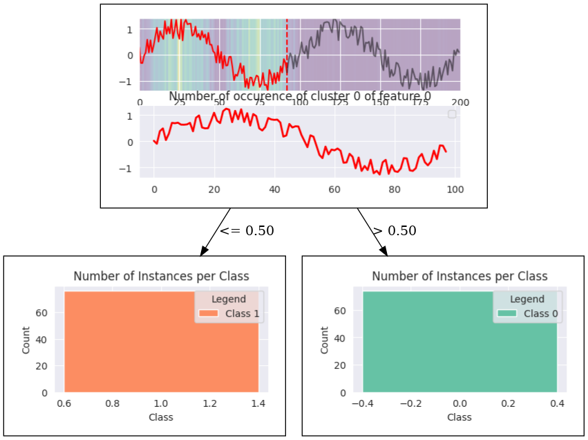
Example of extracting sine wave prototype and explaining class with existence ora absence of a prototype: Jupyter Notebook
Example of extracting sine wave as a prototype end explaining class by difference in frequency of a prototype Jupyter Notebook
The basic usage of the TSProto assuming you have your model trained is straightforward:
from tsproto.models import *
from tsproto.utils import *

#assuming that trainX, trainy and model are given

pe = PrototypeEncoder(clf, n_clusters=2, min_size=50, method='dtw',
                      descriptors=['existance'],
                      jump=1, pen=1,multiplier=None,n_jobs=-1,
                      verbose=1)

trainX, shapclass = getshap(model=model, X=trainX, y=trainy,shap_version='deep',
                        bg_size = 1000,  absshap = True)

#The input needs to be a 3D vector: number of samples, lenght of time-series, number of dimensions (features)
trainXproto = train.reshape((trainX.shape[0], trainX.shape[1],1))
shapclassXproto = shapclass.reshape((shapclass.shape[0], shapclass.shape[1],1))

ohe_train, features, target_ohe,weights = pe.fit_transform(trainXproto,shapclassXproto)

im  = InterpretableModel()
acc,prec,rec,f1,interpretable_model = im.fit_or_predict(ohe_train, features,
                        target_ohe,
                        intclf=None, # if intclf is given, the funciton behaves as predict,
                        verbose=0, max_depth=2, min_samples_leaf=0.05,
                        weights=None)
After the Interpretable model has been created it now can be visualised.